Many detailed examples are available in the examples directory in the github repository. However most contact models will follow a standard work flow:
- Define surface profiles either by reading from file or generating
- If a profile has been read from file, fill in missing data
- Define materials and assign then to the surfaces
- Make a contact model object to coordinate the solution
- Make modelling steps which describe the problem you need to solve
- Add the steps to the model
- Add sub models to the steps as required
- Add output requests to the steps as required
- Check and solve the model
- Post process the results
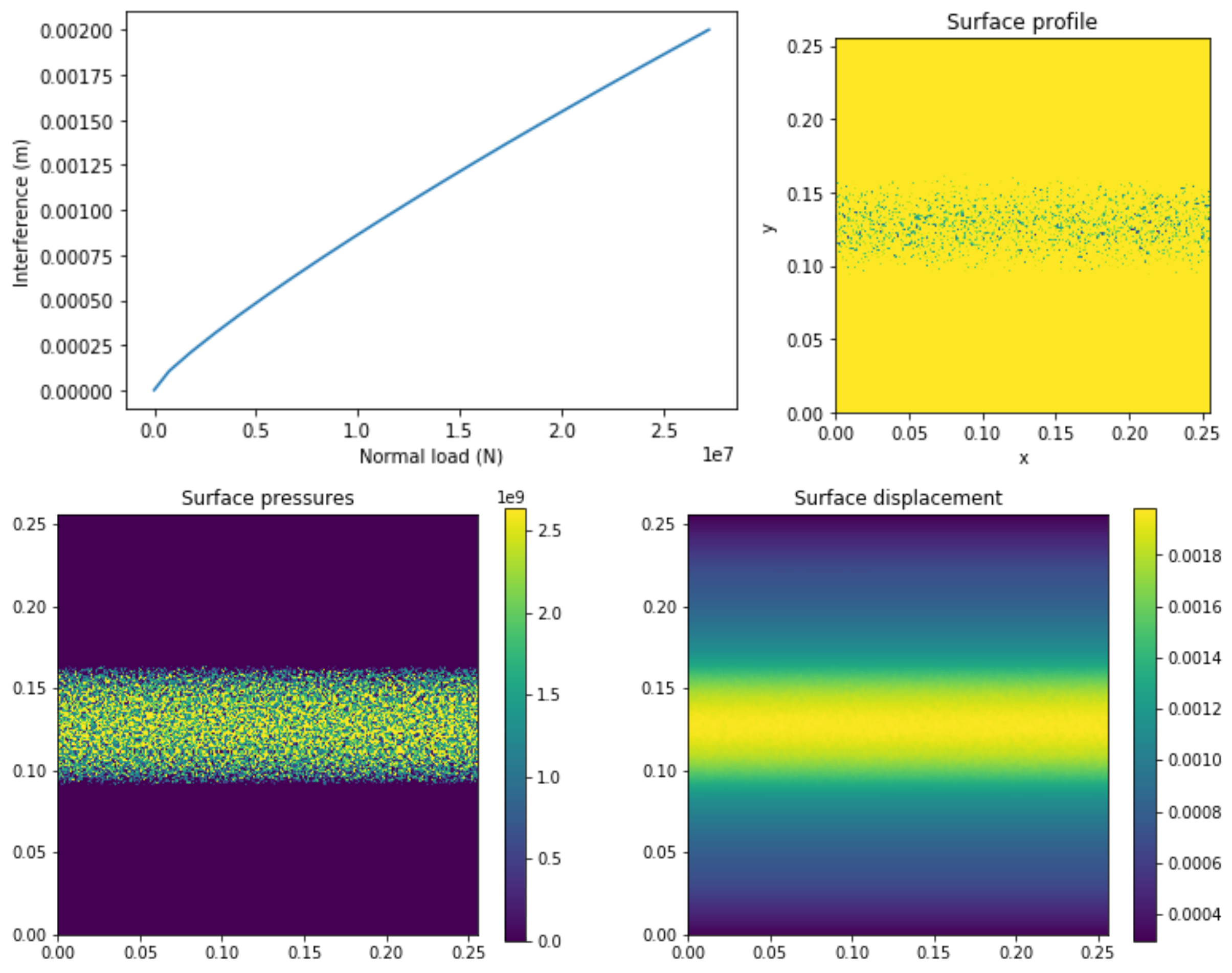
In this simple example a rough cylinder is pressed into a flat plane, materials are elastic but with a maximum allowable pressure to simulate an elastic perfectly plastic material. Where the loads is equal to this maximum load the surfaces are allowed to penetrate each other, here a wear submodel is used to remove this overlap as wear, this permanently changes the surface profiles.
A more detailed description of the decisions behind the code can be found in the example:
import numpy as np
import slippy.surface as s
import slippy.contact as c
# define contact geometry
cylinder = s.RoundSurface((1,np.inf,1), shape=(256,256), grid_spacing=0.001)
roughness = s.HurstFractalSurface(1,0.2,1000, shape=(256, 256), grid_spacing=0.001,
                              generate = True)
combined = cylinder + roughness * 0.00001
flat = s.FlatSurface(shape=(256, 256), grid_spacing=0.001, generate = True)

# define material behaviour and assign to surfaces
yield_stress = 3*np.exp(0.736*0.3)*705e6
material = c.Elastic('steel', properties = {'E':200e9, 'v':0.3}, max_load = yield_stress
combined.material = material
flat.material = material

# make a contact model
my_model = c.ContactModel('qss_test', combined, flat)

# make a modelling step to describe the problem
max_int = 0.002
n_time_steps = 20
my_step = c.QuasiStaticStep('loading', n_time_steps, no_time=True,
                            interference = [max_int*0.001,max_int],
                            periodic_geometry=True, periodic_axes = (False, True))

# add the steps to the model
my_model.add_step(my_step)

# add sub models
wear_submodel = c.sub_models.EPPWear('wear_l', 0.5, True)
my_step.add_sub_model(wear_submodel)

# add output requests
output_request = c.OutputRequest('Output-1',
                                 ['interference', 'total_normal_load',
                                  'loads', 'total_displacement',
                                  'converged'])
my_step.add_output(output_request)

# solve the model
final_result = my_model.solve()
Some examples of results which could be generated from the output of this model are shown below:
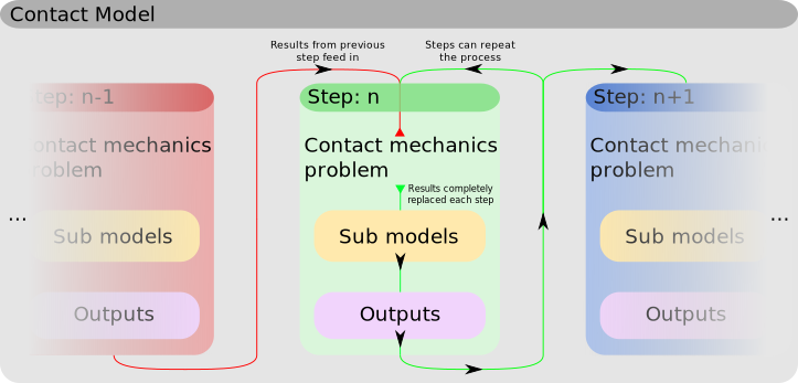
The process of generating a contact model can be difficult to understand, however the process slippy works through in solving a model is relatively simple. For each model step, first any offset (tangential motion) between the surfaces is applied. Next the contact mechanics problem is solved, this should include any processes which need to be two way coupled, for example fluid pressures and deformation in a EHL step.
After this the sub-models are solved, these are one way coupled to the contact mechanics problem in this time step. This means that the result of the contact model can be used in their solution but they cannot impact the solution of the contact mechanics problem in a single time step. Processes like wear, film growth, temperature change, and in some cases tangential contact can be solved in submodels.
Finally the requested outputs are written to file so they can be post processed at a later time. Depending on the step this process can repeat for the same step or the model can move on to the next step: